
The overall scope of the analysis is as follow:
2-1. Class Imbalance Visualization
2-2. Transaction Amounts Distribution
2-3. Time-Based Transaction Patterns
2-3-1. Transaction Frequency Over Time
2-3-2. Fraud Ratio Over Time
2-3-3. Time Gap Between Transactions
2-4. Feature Distribution Analysis (V1–V28)
2-4-0. Strong Features Selection Using Pearson Correlation
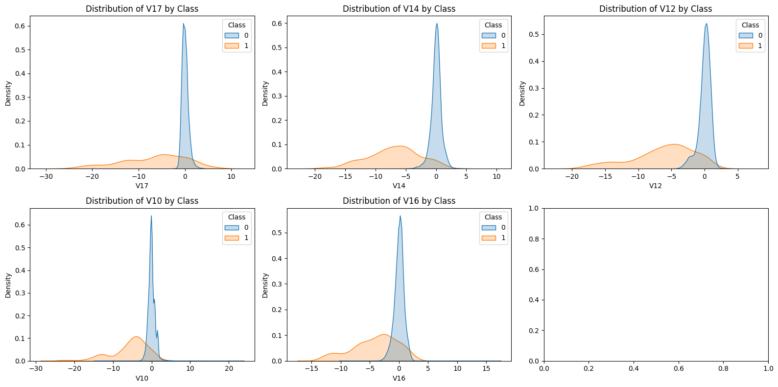
2-4-1. Selected Feature Distributions (Density / Subplots)
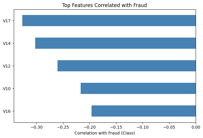
2-4-2. Correlation Analysis (Bar Chart)
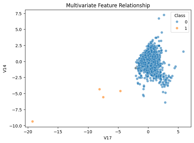
2-4-3. Multivariate Insight (Scatter Plot)
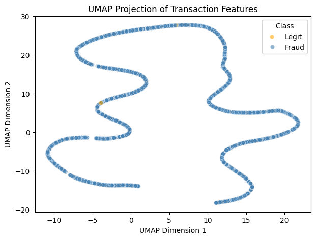
2-4-4. Non-linear Feature Structure Visualization (UMAP)
2-5. Summary of EDA Findings
3. Modeling Preparation and Strategy
3-1. Problem Definition & Evaluation Metrics
3-2. Data Preparation
3-2-1. Handling imbalance
3-2-2. Feature Selection & Scaling
3-3. Model Selection (Random Forest vs. Logistic Regression vs. XGBoost)
3-4. Model Evaluation
3-4-1. Precision–Recall Curve Analysis
3-4-2. Cost-based Evaluation (Business Perspective)
3-5. Insights from Modeling
4. Model Explainability (SHAP)
4-1. Motivation for Model Interpretability
4-2. Global Feature Importance (SHAP Summary)
4-3. Transaction-level Explanation (Single Case SHAP)
4-4. Consistency with EDA Findings
This project explores a publicly available dataset of European credit card transactions in September 2013, with the goal of detecting fraudulent activities using various machine learning models. The dataset is highly imbalanced, containing only 0.17% fraud cases.
We set up the Python environment with commonly used data science libraries, including pandas, numpy, matplotlib, seaborn, scikit-learn, umap, and shap, etc. These libraries support data manipulation, visualization, modeling, and interpretability. Ensuring the proper environment setup allows for reproducible analysis.
The dataset was loaded from the Databricks catalog into a pandas DataFrame. This step converts the raw table into a format suitable for analysis and modeling.
We inspected the first few rows of the dataset and examined its schema, data types, and missing values. This helps identify potential issues and confirms that all expected columns are present.
Numeric features were formatted consistently, and any required scaling or standardization was applied. This ensures that features are on comparable scales, which is important for models that are sensitive to feature magnitude (e.g., Logistic Regression).
Understanding the dataset structure
The Class column indicates transaction type: 0 = legitimate, 1 = fraud. Features V1 to V28 are anonymized via PCA transformations to protect sensitive information. Amount and Time are original transaction features, representing the transaction value and time elapsed since the first recorded transaction, respectively. These steps provide a clean, well-understood dataset, ready for exploratory analysis and modeling.
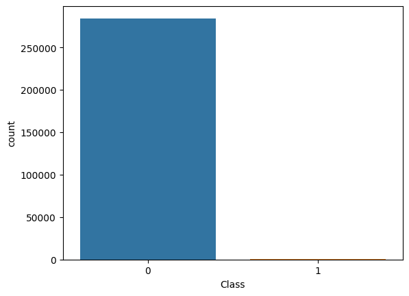
Since fraudulent transactions (Class = 1) are extremely rare, the dataset exhibits a severe class imbalance. Fraud cases account for only 0.17% of all transactions, with 492 frauds out of 284,807 records.
This imbalance has important implications for model evaluation, as accuracy alone would be misleading. Therefore, in the subsequent analysis, we apply balancing techniques to create comparable samples of legitimate and fraudulent transactions for exploratory comparison purposes.
Using a boxplot helps compare the median, spread, and outlier between fraud and non-fraud. Fraudulent transactions sometimes have a narrower or unusual range.

The boxplot shows that fraudulent transactions have a lower median amount than legitimate ones, indicating that fraud often involves smaller transaction values.
However, the fraud class exhibits a larger interquartile range (IQR), suggesting greater variability in transaction amounts among typical fraud cases. This indicates that fraudulent activity does not follow a single consistent amount pattern, but rather spans a wider range of transaction values compared to legitimate transactions.
The histograms display the distribution of transaction amounts.
- The data is divided into 50 intervals along the x-axis. (bins=50)
- The y-axis represents the number of transactions that fall within each amount/time range.
.png)
The histogram illustrates the time elapsed since the first transaction, measured in seconds.
- This is useful for identifying when transactions occur and whether fraudulent activity is more common during certain times of the day.
The distribution of transaction amounts separately for fraudulent and legitimate transactions.
The output explanation for Amount column:
- count 284315.000000 → Total number of transactions analyzed
- mean 88.291022 → Average transaction amount ≈ 88.29
- std 250.105092 → Standard deviation: lots of variation
- min 0.000000 → Smallest transaction was 0.00
- 25% 5.650000 → 25% of transactions were less than 5.65
- 50% 22.000000 → Median amount = 22.00
- 75% 77.050000 → 75% were less than 77.05
- max 25691.160000 → Largest transaction = $25,691.16
Using a histogram shows the frequency distribution of transaction amounts clearly. The fraud cases cluster at specific values, like under $100 or around even dollar amounts
🔍Key insights
- Most legitimate transactions are small (median = $22), but there's a long tail — some are very large.
- The high standard deviation and large max show that the distribution is right-skewed — meaning most transactions are small, but a few big ones pull the average up.
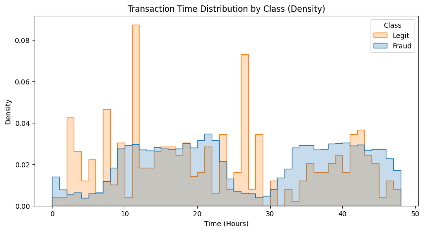
When visualized using density-based distributions, fraudulent transactions exhibit a more uneven temporal distribution, with higher relative density concentrated in specific time windows. In contrast, legitimate transactions display a more uniform temporal density across the observation period.
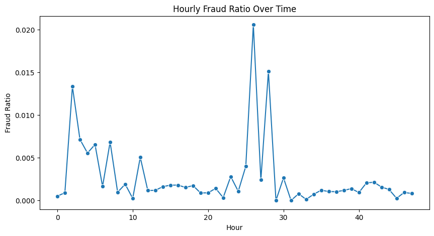
Certain time windows exhibit elevated fraud ratios, suggesting that fraudulent activity is more concentrated during specific periods rather than occurring uniformly over time.
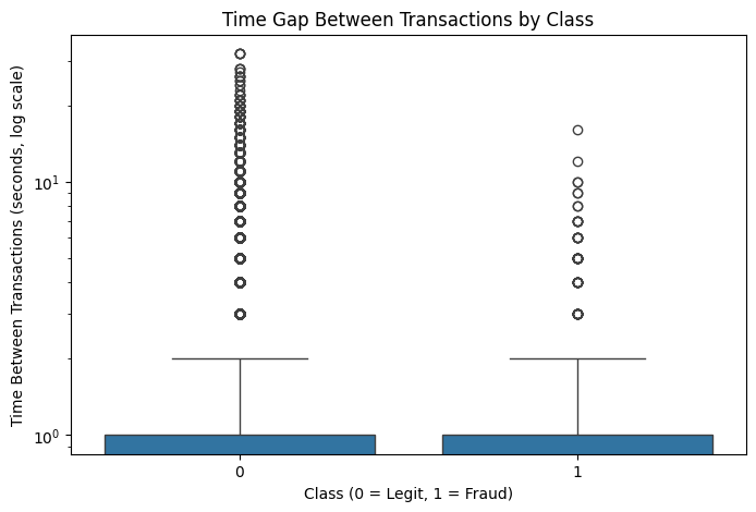
Fraudulent transactions tend to occur in shorter time intervals, indicating burst-like activity patterns compared to legitimate transactions.
Using the Pearson correlation between all numeric features and the target variable (Class), sorts them by absolute strength, and selects the top 5 features most strongly associated with fraudulent transactions. These features are then used for detailed distributional and multivariate analysis.
Correlation analysis highlights a subset of features that are strongly associated with fraudulent transactions, supporting the use of feature-based classification models.
Legitimate transactions (Class 0) tend to fall within a relatively narrow feature range, exhibiting small variations and consistent behavioral patterns. In contrast, fraudulent transactions (Class 1) are more dispersed across the feature space, with some observations lying at extreme values. This deviation from typical patterns highlights anomalous behavior that can be exploited as a predictive signal in classification models.
UMAP was applied to project high-dimensional transaction features into a two-dimensional space. Legitimate transactions form a dense and compact cluster, while fraudulent transactions appear more scattered and partially separated. This suggests that fraud cases deviate from normal transaction patterns across multiple features, providing useful signals for downstream classification models.
Exploratory data analysis reveals that the dataset is extremely imbalanced, with fraudulent transactions accounting for only 0.17% of all records. Transaction amount analysis shows that fraud cases tend to involve smaller amounts, with occasional extreme values, distinguishing them from legitimate transactions.
Time-based analysis indicates that fraudulent transactions are unevenly distributed over the observation period, exhibiting localized temporal patterns rather than a uniform distribution.
Feature distribution and correlation analysis identify several variables (e.g., V14, V17) that exhibit strong associations with fraudulent activity. Multivariate visualization further shows that legitimate transactions cluster within a narrow feature range, while fraud cases are more dispersed and often lie outside typical regions.
Overall, these findings suggest that fraudulent behavior deviates from normal transaction patterns and provides exploitable signals for classification models.
The goal is to identify transactions (Class = 1) from legitimate ones (Class = 0). Given the dataset's severe class imbalance, accuracy alone is insufficient. Therefore, evaluation focuses on metrics such as precision, recall, F1-score, and ROC-AUC to ensure that fraudulent transactions are correctly detected.
The dataset exhibits extreme class imbalance, with fraudulent transactions representing only 0.17% of all records. To prevent the model from being biased toward the majority class, we applied oversampling of the minority class by Synthetic Minority Oversampling Technique (SMOTE), and used class-weight adjustments in tree-based models. This ensures that the classifier gives sufficient attention to the rare fraudulent cases while training.
Based on the EDA, we selected the top features that show the strongest correlation with the target variable (Class). These features capture meaningful distributional differences between fraudulent and legitimate transactions.
For linear models, features were standardized to have zero mean and unit variance, whereas tree-based models were trained on raw features, as they are insensitive to feature scaling.
We evaluated several classification algorithms suitable for imbalanced datasets.
- Random Forest and XGBoost were chosen as tree-based models capable of capturing non-linear relationships and complex interactions.
- Logistic Regression was included as a baseline linear model for comparison.
Class weights were adjusted to balance the contribution of minority class samples, which improves the model’s ability to detect fraudulent transactions.
Models were evaluated on a held-out test set using metrics appropriate for highly imbalanced data. Since accuracy can be misleading due to the low prevalence of fraud, the following metrics were emphasized:
- Recall: the proportion of fraudulent transactions correctly identified
- Precision: the proportion of predicted fraud cases that are truly fraudulent
- F1-score: the harmonic mean of precision and recall
- ROC-AUC: overall separability between legitimate and fraudulent classes
Confusion matrices, ROC curves, and Precision–Recall (PR) curves were used to assess model performance. While ROC curves provide a general measure of a model’s discriminative ability, PR curves are more informative in highly imbalanced settings, as they focus on the trade-off between precision and recall for the minority (fraud) class. This evaluation framework enables a more realistic assessment of both fraud detection capability and prediction reliability.
Given the extreme class imbalance, the Precision–Recall (PR) curve provides a more informative evaluation than ROC-AUC.
The PR curve highlights the trade-off between detecting fraudulent transactions (recall) and minimizing false alarms (precision).
A high ROC-AUC may still correspond to poor precision for the minority class, making PR analysis critical for fraud detection tasks.
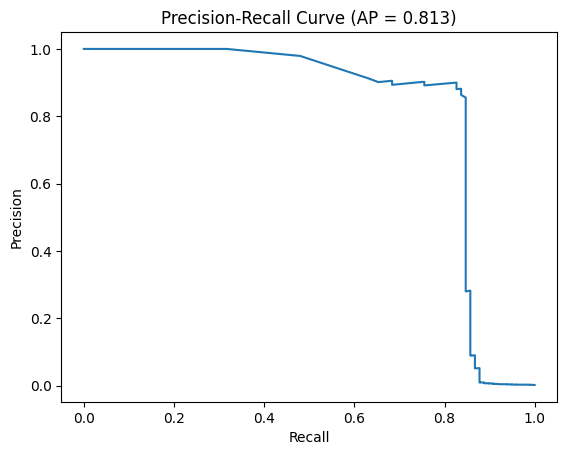
The Precision–Recall curve yields an Average Precision (AP) score of 0.813, indicating strong performance in identifying fraudulent transactions under severe class imbalance. Since AP summarizes precision across all recall levels, this result suggests that the model maintains high prediction reliability even as recall increases.
Compared to the extremely low baseline precision determined by fraud prevalence, the achieved AP demonstrates substantial improvement over random guessing and highlights the model’s effectiveness in practical fraud detection.
To reflect real-world impact, we introduced a cost-sensitive evaluation assuming a false negative cost of $500 and a false positive cost of $5.
This analysis demonstrates that models with higher recall for fraud can significantly reduce overall financial loss, even at the expense of lower precision.
--- Random Forest ---
precision recall f1-score support
0 1.00 1.00 1.00 56864
1 0.47 0.85 0.61 98
accuracy 1.00 56962
macro avg 0.74 0.92 0.80 56962
weighted avg 1.00 1.00 1.00 56962
ROC-AUC: 0.9510560643081093
False Negatives (FN): 15
False Positives (FP): 93
Total Cost: $7,965
--- Logistic Regression ---
precision recall f1-score support
0 1.00 0.98 0.99 56864
1 0.06 0.90 0.12 98
accuracy 0.98 56962
macro avg 0.53 0.94 0.55 56962
weighted avg 1.00 0.98 0.99 56962
ROC-AUC: 0.9683494740045708
False Negatives (FN): 10
False Positives (FP): 1308
Total Cost: $11,540
--- XGBoost ---
precision recall f1-score support
0 1.00 0.96 0.98 56864
1 0.03 0.88 0.07 98
accuracy 0.96 56962
macro avg 0.52 0.92 0.52 56962
weighted avg 1.00 0.96 0.98 56962
ROC-AUC: 0.9395749471707647
False Negatives (FN): 12
False Positives (FP): 2423
Total Cost: $18,115
Among the three evaluated models, Random Forest achieved the best balance between recall (0.85) and precision (0.47) for fraud detection, successfully identifying most fraudulent transactions while limiting false positives.
Logistic Regression and XGBoost achieved slightly higher recall (0.90 and 0.88, respectively), but their extremely low precision led to a large number of false positives, substantially increasing operational cost.
When incorporating cost-based evaluation, Random Forest resulted in the lowest total cost, despite not having the highest ROC-AUC. This indicates that Random Forest provides the most practical and cost-effective performance for fraud detection in this highly imbalanced dataset.
Confusion matrix analysis provides insight into the types of errors made by each model. In fraud detection, false negatives represent missed fraudulent transactions with direct financial loss, while false positives incur operational costs due to unnecessary transaction reviews.
Among the evaluated models, Logistic Regression and XGBoost demonstrated strong overall separability and high recall; however, their extremely low precision resulted in a large number of false positives, significantly increasing operational cost and limiting practical usability. In contrast, Random Forest achieved the lowest total cost by maintaining high fraud recall while limiting false positives, making it the most practical model for deployment.
These results are consistent with EDA findings, confirming that fraudulent transactions tend to deviate from typical feature ranges rather than follow simple linear patterns. Consequently, non-linear, tree-based models are better suited to capture these complex behaviors.
Overall, these insights emphasize the importance of balancing recall and precision, leveraging EDA-driven feature understanding, and incorporating cost-based evaluation to guide practical model selection in real-world fraud detection.
While predictive performance is critical in fraud detection, model transparency is equally important for trust, regulatory compliance, and human-in-the-loop decision making. Therefore, SHAP was applied to interpret the predictions of the selected Random Forest model at both global and transaction levels.
Although predictive performance is critical in fraud detection, model interpretability is equally important for trust, regulatory compliance, and operational decision-making. Fraud detection systems are often used in high-stakes environments where incorrect predictions may lead to financial loss or poor customer experience. Therefore, understanding which features drive model predictions is essential before deployment.
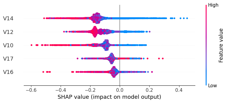
From the SHAP summary plot, the top features influencing fraud prediction are V14, V12, V10, V17, and V16.
Most high feature values (red points) have negative SHAP values, indicating they decrease the predicted fraud probability, whereas most low feature values (blue points) have positive SHAP values, indicating they increase the predicted fraud probability.
This suggests that, for these features, transactions with unusually low values are more likely to be classified as fraud by the model, while high values are associated with normal transactions.
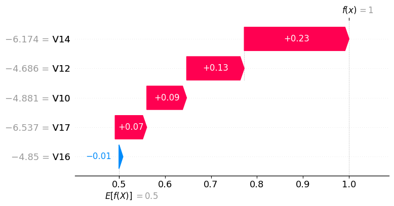
In the SHAP waterfall plot for this single transaction, V14, V12, V10, and V17 contribute positively to the predicted fraud probability, with SHAP values of 0.23, 0.13, 0.09, and 0.07, respectively. V16 has a slight negative contribution of -0.01, indicating it slightly reduces the fraud probability. Overall, the model classifies this transaction as high-risk primarily due to the strong positive contributions from V14, V12, V10, and V17.
The SHAP analysis reinforces insights obtained from the EDA. Features identified as highly discriminative during exploratory analysis also exhibit strong contributions in the trained Random Forest model. This consistency increases confidence that the model is learning meaningful behavioral patterns rather than spurious correlations.
The feature ranking based on SHAP values differs from the simple correlation analysis because correlation measures only the linear relationship between each feature and the target, independently of other features. SHAP, on the other hand, captures the contribution of each feature within the trained Random Forest model, accounting for non-linear interactions and dependencies among features. As a result, some features with moderate correlation, such as V14, may appear more important to the model than features with higher linear correlation, such as V17.
This observation also aligns with the non-linear structures revealed by UMAP and multivariate scatter plots in the EDA, further confirming that the Random Forest model effectively captures complex feature patterns.
This project presents a comprehensive exploratory data analysis (EDA) and machine learning approach to credit card fraud detection. We analyzed transaction amount and temporal patterns to identify behavioral differences between legitimate and fraudulent transactions, and addressed severe class imbalance through stratified data splitting and class-weighted learning. Multiple classification models, including Random Forest, XGBoost, and Logistic Regression, were evaluated using metrics appropriate for imbalanced data, such as precision, recall, F1-score, and ROC-AUC.
Tree-based models, particularly Random Forest, achieved a strong balance between fraud detection recall and prediction reliability. Their superior performance reflects the ability to capture non-linear relationships and complex interactions among transaction features. Furthermore, SHAP analysis was applied to interpret the Random Forest model, revealing which features most strongly influence predictions at both the global level and for individual transactions. Incorporating cost-based evaluation highlights that Random Forest not only performs well statistically, but also minimizes potential financial loss, reinforcing its practical applicability.
Overall, the findings demonstrate that fraudulent transactions tend to deviate from normal behavioral patterns and that non-linear, interpretable models, guided by EDA-driven feature understanding, are well suited to detect such complex characteristics.
📌 Streamlit (HF Space): Credit Card Fraud Detection 💳 $pot credit card fraud in a few clicks
📌 GitHub: github.com/JYUN-YI/credit-card-fraud-detection
📌 Data Sources: Kaggle Credit Card Fraud Detection Dataset